the tropopause

[historical remarks]   [why is it so sharp?]

for comments/suggestions/questions please contact me at tbirner.work'at'gmail'dot'com

historical remarks

New: my English translation of Richard Assmann's 1902 article, in which he describes his discovery of the upper inversion. I have added a graphical version of his temperature data. The original German article can be found at Geoff Vallis' website of historical papers.

Many more details than described below can be found in Hoinka, 1997: The tropopause: discovery, definition and demarcation, Meteorol. Zeitschrift, N. F. 6, 281-303. The images shown below are taken from Hoinka (1997).

Stories of discoveries are always fascinating and the one about the tropopause is no exception. And as in many other cases the tropopause was discovered more or less by chance and was discarded as a measurement error at first.

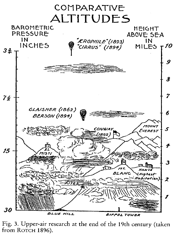
200 years ago people knew from the temperature difference between mountain tops and valleys that temperature drops with height at roughly 7 K/km (this is about 7.8 F/mi). It is a simple exercise to realize that this would lead to 0 K (= -273.15 C or -459.67 F, i.e. absolute zero) at an altitude of 40 km (assuming a surface temperature of 280 K = 44 F).

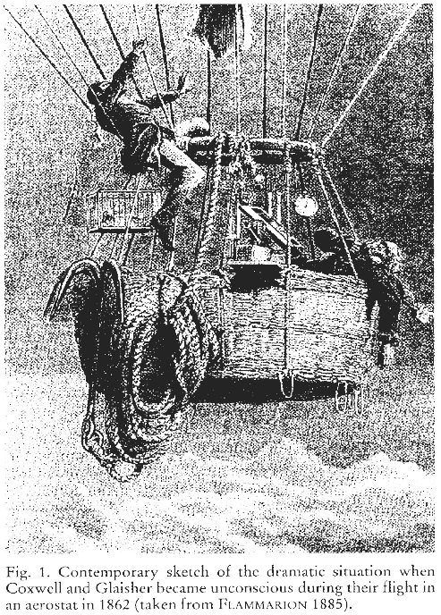Discovering the 3rd dimension in the second half of the 19th century. Coxwell and Glaisher (image on the right) became unconscious as they reached altitudes of about 10 km during their flight in 1862!

So something must be happening to the temperature distribution before it reaches absolute zero. It was when ballon soundings of temperature and pressure first came up toward the end of the 19th century (mainly in France and Germany) that measurements were obtained at large enough altitudes to make possible the discovery of the tropopause (and with it of the stratosphere). One of the first such ballons launched in November 1896 by the Frenchman L. Teisserenc de Bort in Paris reached 14 km and measured constant temperature between about 12 and 14 km. However, this isothermal behavior was discarded as a measurement error and instead temperature was extrapolated above 12 km using the typical temperature decrease below 12km!

It took Teisserence de Bort almost 10 years and more than 200 collected soundings to trust his results enough and have the heart to report his results to the French Acadamy of Sciences in April 1902 and announce the discovery of an isothermal layer ("zone isotherme" in french). As little as three days(!) later the German R. Assmann announced essentially the same discovery to the German Academy of Science referring to the isothermal layer as upper inversion.

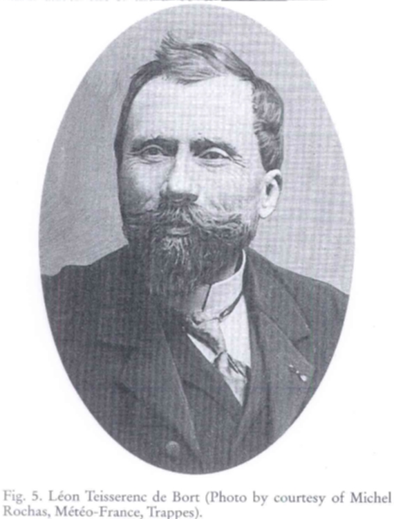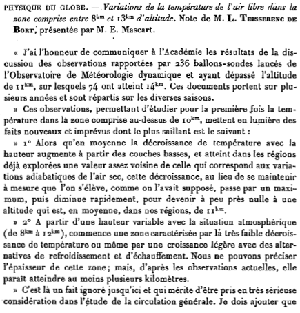Teisserenc de Bort and the first page of his report on "Variations in the temperature of the free air in the zone between 8 and 13 km altitude". Remarkably, de Bort already noted variations in tropopause height associated with upper level cyclones (lower tropopause) and upper level anticyclones (higher tropopause).

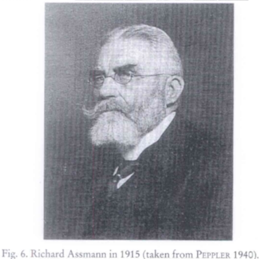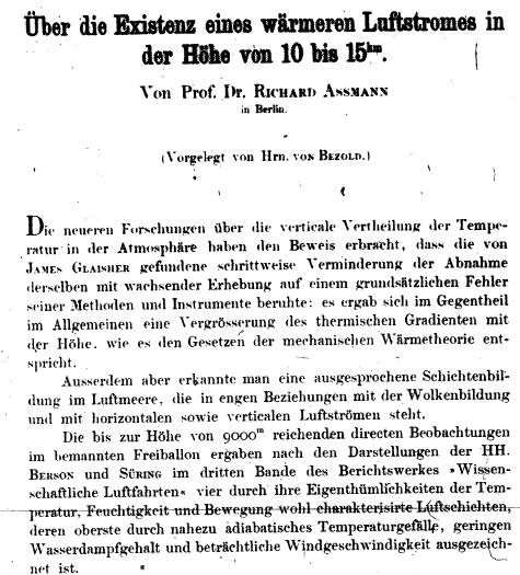Richard Assmann and the first page of his report "On the existence of a warmer airflow at heights from 10 to 15 km". Interesting side-note: as we now know Assmann's notion of "upper inversion" (that is, a change from decreasing to increasing temperature at the bottom of the stratosphere) is somewhat closer to the truth than de Bort's "isothermal layer" (although de Bort also remarked that the stratosphere sometimes started with an inversion).

The isothermal layer as discovered by Teisserenc de Bort and Assmann represents the first few kilometers of what we now call the stratosphere (a term introduced by Teisserenc de Bort around 1908, as was troposphere for the lowest part of the atmosphere). And as stated above the lower boundary of the stratosphere is called the tropopause (a term popularized by Sir Napier Shaw around 1920).

why is it so sharp?

Observational studies using data with fine vertical resolution (100 m or better) have documented that the transition from troposphere to stratosphere is on average extremely sharp, in fact almost step-like (see graph below). The best way to quantify this is to look at a measure of the degree of stratification of the atmosphere. This seems very natural given the notion of the troposphere to represent a well-mixed layer (tropos is greek for "to turn") with weak stratification and the stratosphere *surprise* to represent a more strongly stratified layer.

The degree of stratification measures how hard it is for a fluid (air) parcel to travel vertically. This is directly measured by the so-called buoyancy frequency - this is the frequency with which an air parcel would oscillate if displaced from its equilibrium position. For stronger stratification (stratosphere) the air parcel will oscillate faster (higher buoyancy frequency) whereas for weaker stratification (troposphere) the air parcel will oscillate slower (lower buoyancy frequency).

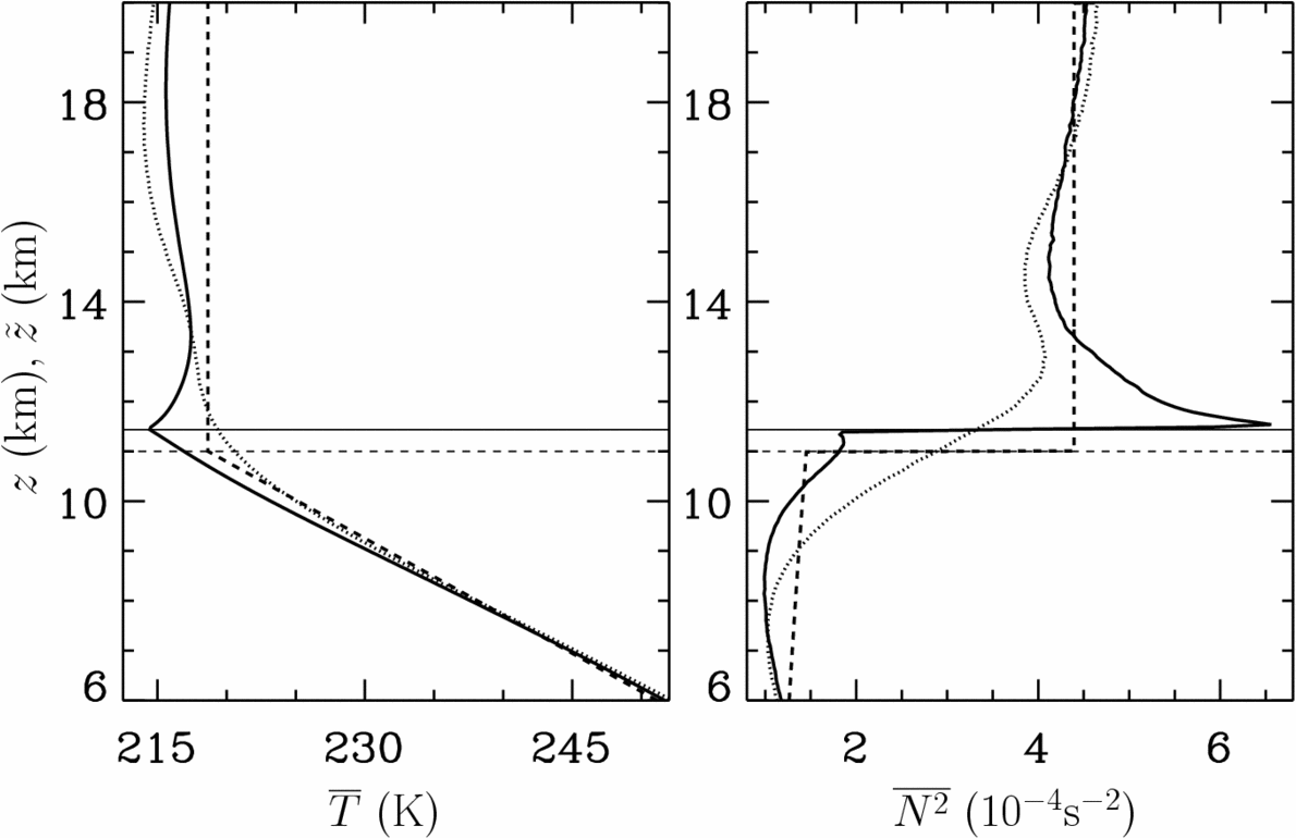Climatology representative for northern mid-latitudes (about 45 N) of temperature (left) and buoyancy frequency squared (right) between 6-20 km altitude. 5 years (1998-2002) of radiosonde data with a vertical resolution of about 50 m have been used. Full lines: tropopause-based (TB) average (see illustration further below), dotted lines: conventional averages, dashed lines: U.S. standard atmosphere. The horizontal line marks the average position of the tropopause. Note the abrupt jump in stratification (as measured by the buoyancy frequency) at the tropopause seen in the tropopause-based average. Similar pictures arise at other latitudes. Taken from Birner (2006)

The above graph shows that when temperature is simply/conventionally averaged the transition between troposphere and stratosphere appears very smooth and gradual. Anybody who has looked at individual temperature soundings will confirm that this smooth transition does not represent the transition found in most individual soundings. The problem with the conventional average is that the tropopause level fluctuates quite strongly in time and in space. In mid-latitudes the tropopause can be located as low as 5 km one day and as high as 15 km a week later (even though that would represent an extreme case)! This range of minimum/maximum tropopause heights of 10 km is as large as the average tropopause height itself!

The way out is to compute the averages relative to the position of the tropopause (called tropopause-based average above). This is illustrated below (taken from Birner (2006)).

	Conventional average. Left: three hypothetical temperature profiles with clearly marked individual tropopause levels at different altitudes. Right: when averaged the sharpness of the individual tropopause levels is lost since each individual tropopause level enters the average at a different altitude.
	Tropopause-based average. Left: the same three hypothetical temperature profiles as above. Right: this time, the average is computed relative to the tropopause level, that is by averaging temperature at given distances from the tropopause level. This way the characteristic temperature structure around the tropopause of the individual profiles is preserved in the average.

But to come back to the original question: why is the transition between troposphere and stratosphere so abrupt, why is the tropopause so sharp? And further: why does stratification maximize in the lowest part of the stratosphere (see maximum in buoyancy frequency just above the tropopause)? Well, this is the part we still don't fully understand. A few ideas/theories have been put forward relating tropopause sharpness to specific features of upper level cyclones and anticyclones, radiation, or large-scale circulations. They all seem to explain at least part of the observed temperature structure but none of them is fully conclusive. For more on this see, e.g., the UTLS review paper, section 3.2 therein.